First Python 3 Geospatial Book

Chapter 8 demonstrates advanced geospatial modeling 

using Python 3 to create a color hillshade like this as well 

as several other commonly used real-world examples.

The second edition of "Learning Geospatial Analysis with Python" is now available!  To my

knowledge, this is the first book dedicated to Python 3 and geospatial analysis.
The book opens with the incredible story of how the grass-roots, open-source Ushahidi project stopped the Ebola epidemic in its tracks. It continues with one of the best histories of geospatial technologies you'll find.  The chapters closes with you creating a complete GIS using only 60 lines of Python code!

Chapter 2 teaches you the data types you'll encounter on your journey into geospatial analysis. Chapter 3 surveys commonly-used geospatial software to give you the context you need to navigate geospatial solutions.  Chapter 4 covers Python geospatial tools.  Chapter 5 dives into GIS operations with Python.  Chapter 6 teaches you Python 3 remote sensing techniques.  And Chapter 7 is a one-of-a-kind examination of elevation data with several examples.  Chapter 8 covers complete geospatial modeling techniques for real-world situations like the color hillshade in this post.  Chapter 9 explores the emerging world of real-time tracking data.  And Chapter 10 pulls the whole book together to build a complete application.

You get over 100 examples with test data and code plus explanations in either a print or e-book available from Packt Publishing or pretty much any other online book seller.  If you get the print book, or if you just want to see the images, I've made them available as a zip file download here.

While many books in this category do a great job of covering Python APIs to different libraries, this book focuses as much as possible on algorithms to show you the raw calculations that make up geospatial analysis.  This approach allows you to not only run the examples but break things down line by line to see how it works and recombine pieces of code on your own to go beyond the book.

Click the link on the right to check it out on Amazon!

CSV to Shapefile

Converting a comma-separated value (CSV) file to a shapefile comes up a lot on forums.  This post is a quick example of transforming a CSV file to a shapefile using PyShp and the built-in Python csv module.  CSV files usually contain fields separated by commas but might also use some other delimiter such as a pipe "|" or tab.  The csv module defaults to commas but will let you set other delimiters. Here is the file we'll be using that I slightly modified from a GIS StackExchange question flagged as duplicate:

Name,Area,geometry
town,123,"POLYGON((73.953695297241 15.3555421329,73.951292037964 15.314816978733,73.986654281616 15.310015523128,73.982191085815 15.345775441645,73.953695297241 15.3555421329))"
forest,500,"POLYGON((73.938202857971 15.34362339739,73.944897651672 15.343375083164,73.943438529968 15.341554103151,73.942408561707 15.337084357624,73.941378593445 15.340395289421,73.937001228333 15.341471330955,73.938202857971 15.34362339739))"
lake,800,"POLYGON((73.995494842529 15.291305352455,73.999614715576 15.287165708411,74.000301361084 15.283357163686,73.997898101807 15.281701253096,73.99377822876 15.282363618901,73.99377822876 15.284516293317,73.992576599121 15.287496882943,73.992919921875 15.289815090018,73.995494842529 15.291305352455))"

This notional CSV has three fields for the name of the feature, the area, and the geometry. The geometry consists of a WKT string describing the polygon coordinates. The polygons contain varying numbers of coordinates and the x,y values are separated by commas. None of this will confuse the csv module because they are contained in strings. The code is very simple. We use the csv module to access the data as rows and fields. Then we manually parse the coordinates as strings. And finally we write the shapefile in a loop:

import csv
import shapefile

# Create a polygon shapefile writer
w = shapefile.Writer(shapefile.POLYGON)

# Add our fields
w.field("NAME", "C", "40")
w.field("AREA", "C", "40")

# Open the csv file and set up a reader
with open("sample.csv") as p:
    reader = csv.DictReader(p)
    for row in reader:
        # Add records for each polygon for name and area
        w.record(row["Name"], row["Area"])
        # parse the coordinate string
        wkt = row["geometry"][9:-2]
        # break the coordinate string in to x,y values
        coords = wkt.split(",")
        # set up a list to contain the coordinates
        part = []
        # convert the x,y values to floats
        for c in coords:
            x,y = c.split(" ")
            part.append([float(x),float(y)])
        # create a polygon record with the list of coordinates.
        w.poly(parts=[part])

# save the shapefile!
w.save("polys.shp")

You can download the code and CSV file on GitHub.

Basic Image Change Detection in QGIS and Python

Change detection allows you to automatically highlight the differences between two images in the same area if they are properly orthorectified. We'll do a simple difference change detection on two images, which are several years apart, to see the differences in urban development and the natural environment.  Change detection algorithms can become quite sophisticated.  However at the most basic level, you can do a simple, literal mathematical difference between the pixel values in the two images.  That basic image difference is exactly what we'll do in this example.   This recipe is from my book, the"QGIS Python Programming Cookbook".   I show how do the same operation using the gdalnumeric module outside of QGIS in my other book "Learning Geospatial Analysis with Python".

We're going to start with two aerial images taken several years apart.  We'll subtract the before image from the after image and and visualize the result using a color ramp.

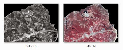
The before and after aerial photos we'll use for this recipe.
Click for  a larger version.

Getting ready

You will need a data directory to store the source images.  I usually create a directory named qgis_data for these types of experiments.  You can download the two images used in this example from https://github.com/GeospatialPython/qgis/blob/gh-pages/change-detection.zip?raw=true and put them in a directory named change-detection in the rasters directory of your qgis_data directory. Note that the file is 55 megabytes, so it may take several minutes to download.  Also, we'll step through this script a few lines at a time.  It's meant to be run in the QGIS Python Console.  You can download the entire script here: https://github.com/GeospatialPython/qgis/raw/master/4985_08_15-change.py

How to do it...

We'll use the QGIS raster calculator to subtract the images in order to get the difference, which will highlight significant changes. We'll also add a color ramp shader to the output in order to visualize the changes. To do this, we need to perform the following steps:

First, we need to import the libraries that we need in to the QGIS console:

from PyQt4.QtGui import *
from PyQt4.QtCore import *
from qgis.analysis import *

Now, we'll set up the path names and raster names for our images:

before = "/Users/joellawhead/qgis_data/rasters/change-detection/before.tif"
|after = "/Users/joellawhead/qgis_data/rasters/change-detection/after.tif"
beforeName = "Before"
afterName = "After"

Next, we'll establish our images as raster layers:

beforeRaster = QgsRasterLayer(before, beforeName)
afterRaster = QgsRasterLayer(after, afterName)

Then, we can build the calculator entries:

beforeEntry = QgsRasterCalculatorEntry()
afterEntry = QgsRasterCalculatorEntry()
beforeEntry.raster = beforeRaster
afterEntry.raster = afterRaster
beforeEntry.bandNumber = 1
afterEntry.bandNumber = 2
beforeEntry.ref = beforeName + "@1"
afterEntry.ref = afterName + "@2"
entries = [afterEntry, beforeEntry]

Now, we'll set up the simple expression that does the math for remote sensing:

exp = "%s - %s" % (afterEntry.ref, beforeEntry.ref)

Then, we can set up the output file path, the raster extent, and pixel width and height:

output = "/Users/joellawhead/qgis_data/rasters/change-detection/change.tif"
e = beforeRaster.extent()
w = beforeRaster.width()
h = beforeRaster.height()

Now, we perform the calculation:

change = QgsRasterCalculator(exp, output, "GTiff", e, w, h, entries)
change.processCalculation()

Finally, we'll load the output as a layer, create the color ramp shader, apply it to the layer, and add it to the map, as shown here:

lyr = QgsRasterLayer(output, "Change")
algorithm = QgsContrastEnhancement.StretchToMinimumMaximum
limits = QgsRaster.ContrastEnhancementMinMax
lyr.setContrastEnhancement(algorithm, limits)
s = QgsRasterShader()
c = QgsColorRampShader()
c.setColorRampType(QgsColorRampShader.INTERPOLATED)
i = []
qri = QgsColorRampShader.ColorRampItem
i.append(qri(0, QColor(0,0,0,0), 'NODATA'))
i.append(qri(-101, QColor(123,50,148,255), 'Significant Itensity Decrease'))
i.append(qri(-42.2395, QColor(194,165,207,255), 'Minor Itensity Decrease'))
i.append(qri(16.649, QColor(247,247,247,0), 'No Change'))
i.append(qri(75.5375, QColor(166,219,160,255), 'Minor Itensity Increase'))
i.append(qri(135, QColor(0,136,55,255), 'Significant Itensity Increase'))
c.setColorRampItemList(i)
s.setRasterShaderFunction(c)
ps = QgsSingleBandPseudoColorRenderer(lyr.dataProvider(), 1, s)
lyr.setRenderer(ps)
QgsMapLayerRegistry.instance().addMapLayer(lyr)

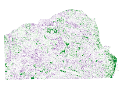
You should end up with the following image.  As a general rule of thumb, green shows area of change where something was built or trees were removed, and purple areas show where a road or structure was likely moved.  There is lots of noise and false positives.  But the algorithm does very well in areas of significant change.

BAM! Change detection! Click for larger version

How it works...

If a building is added in the new image, it will be brighter than its surroundings. If a building is removed, the new image will be darker in that area. The same holds true for vegetation, to some extent.

Here is a close up of an area of intense change that demonstrates what we're talking about.  In the following image, a single softball field was expanded into an entire softball field complex.  In the upper left of the image you can see where the trees were cleared and bright-green grass and dirt infields were added.  In the purple area in the lower right of the image you can see where the original field was rotated.  Further in that direction, you can see some of the noise where the intensity changed between the images but it doesn't have much meaning. However if you zoomed out, the areas of significant change stand out very clearly which is usually the point of this kind of analysis:

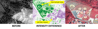
Looking at these softball fields close up really
shows what's happening. Click for larger version

Summary

The concept is simple. We subtract the older image data from the new image data. Concentrating on urban areas tends to be highly-reflective and results in higher image pixel values.

Clipping a Shapefile in Pure Python

In a previous post, I showed how to use pure Python to subset a shapefile by attributes.  That method is fast if the attributes define the data you want to clip.  But sometimes you need to clip data spatially.

In this post, we'll clip a road shapefile using bounding boxes.  This is the simplest type of clip.  In a future post, I'll demonstrate how to use irregular polygons which is more complex.  However the ingredients I'll use for that recipe are already on this blog (this post + PyShp + the ray-casting point-in-polygon algorithm).

Here's our goal for this example. We have a shapefile with the major roads of the United States which you can download a sample dataset here. We want to use a simple bounding box to subset the roads for Puerto Rico. Here's a view of part of that shapefile including Florida and Puerto Rico in the lower right of the image.  It gives you a good idea of the density and number of records in this data.

Each road in the shapefile has its own shape record with the bounding box of the road in the record header.  We'll just do a simple bounding box comparison to isolate the roads within our desired bounding box and then write those results to a new shapefile.  You'll also need the latest version of PyShp which provides the newer iterShapeRecords() method to provide and efficient iterator for both the shapes and the dbf attributes in a single object:

import shapefile

# Create a reader instance for our US Roads shapefile
r = shapefile.Reader("roadtrl020") 

# Create a writer instance copying the reader's shapefile type
w = shapefile.Writer(r.shapeType)

# Copy the database fields to the writer
w.fields = list(r.fields)

# Our selection box that contains Puerto Rico
xmin = -67.5
xmax = -65.0
ymin = 17.8
ymax = 18.6

# Iterate through the shapes and attributes at the same time
for road in r.iterShapeRecords():
    # Shape geometry
    geom = road.shape
    # Database attributes 
    rec = road.record
    # Get the bounding box of the shape (a single road)
    sxmin, symin, sxmax, symax = geom.bbox
    # Compare it to our Puerto Rico bounding box.
    # go to the next road as soon as a coordinate is outside the box
    if sxmin <  xmin: continue
    elif sxmax > xmax: continue
    elif symin < ymin: continue
    elif symax > ymax: continue
    # Road is inside our selection box.
    # Add it to the new shapefile
    w._shapes.append(geom)
    w.records.append(rec)
    
# Save the new shapefile! (.shp, .shx, .dbf)
w.save("Puerto_Rico_Roads")

And here's our result!

Yes, there are dozens of tools and libraries that will do the same thing.  But this is the only solution in the entire (known) universe that is implemented in pure Python.  You don't need any compiled C code.  If you have the ability to run Python 2 or 3, you can run this without any additional system permissions.  It will run where most other libraries won't and when that's what your requirements are, nothing else will do!

Geolocating Photos in QGIS

Photos taken with GPS-enabled cameras, including smartphones, store location information in the header of the file, in a format called EXIF tags. These tags are largely based on the same header tags used by the TIFF image standard. If you have a directory full of photos, you can easily sort them by date or by name.  But if you want to sort them by location, only a map will do.  In this recipe, we'll use these tags to create locations on a map in QGIS for some photos and provide links to open them. 

Getting ready

You need to make sure you have QGIS installed as well as the Python Imaging Library (PIL) for the Python distribution that QGIS uses.  QGIS should already have PIL included. You can download some sample geotagged images here or you can use any photo taken outdoors with your smartphone.  Unzip these photos and place them in a directory accessible to QGIS.

How to do it...

PIL can parse EXIF tags. We will gather the file names of the photos, parse the location information, convert it to decimal degrees, create the point vector layer, add the photo locations, and add a QGIS action link to the attributes. To do this, we need to perform the following steps:

In the QGIS Python Console, import the libraries that we'll need, including the Image module (PIL) and its ExifTags module for parsing image data and the glob module for doing wildcard file searches:

import glob
import Image
from ExifTags import TAGS

Next, we'll create a function that can parse the header data:

def exif(img):
   exif_data = {}
   try:  
       i = Image.open(img)
       tags = i._getexif()
       for tag, value in tags.items():
         decoded = TAGS.get(tag, tag)
           exif_data[decoded] = value
   except:
       pass
return exif_data

Now, we'll create a function that can convert degrees-minute-seconds to decimal degrees, which is how coordinates are stored in JPEG images:

def dms2dd(d, m, s, i):
   sec = float((m * 60) + s)
   dec = float(sec / 3600)
   deg = float(d + dec)
   if i.upper() == 'W':
       deg = deg * -1
   elif i.upper() == 'S':
       deg = deg * -1
   return float(deg)

Next, we'll define a function to parse the location data from the header data:

def gps(exif):
   lat = None
   lon = None
   if exif['GPSInfo']:      
       # Lat
       coords = exif['GPSInfo']
       i = coords[1]
       d = coords[2][0][0]
       m = coords[2][1][0]
       s = coords[2][2][0]
       lat = dms2dd(d, m ,s, i)
       # Lon
       i = coords[3]
       d = coords[4][0][0]
       m = coords[4][1][0]
       s = coords[4][2][0]
       lon = dms2dd(d, m ,s, i)
return lat, lon

Next, we'll loop through the photos directory, get the file names, parse the location information, and build a simple dictionary to store the information, as follows:

photos = {}
photo_dir = "/Users/joellawhead/qgis_data/photos/"
files = glob.glob(photo_dir + "*.jpg")
for f in files:
   e = exif(f)
   lat, lon = gps(e)
 photos[f] = [lon, lat]

Now, we'll set up the vector layer for editing:

lyr_info = "Point?crs=epsg:4326&field=photo:string(75)"
vectorLyr = QgsVectorLayer(lyr_info, \"Geotagged Photos" , "memory")
vpr = vectorLyr.dataProvider()

We'll add the photo details to the vector layer:

features = []
for pth, p in photos.items():
   lon, lat = p
   pnt = QgsGeometry.fromPoint(QgsPoint(lon,lat))
   f = QgsFeature()
   f.setGeometry(pnt)
   f.setAttributes([pth])
   features.append(f)
vpr.addFeatures(features)
vectorLyr.updateExtents()

Now, we can add the layer to the map and make the active layer:

QgsMapLayerRegistry.instance().addMapLayer(vectorLyr)
iface.setActiveLayer(vectorLyr)
activeLyr = iface.activeLayer()

Finally, we'll add an action that allows you to click on it and open the photo.  Actions are a simple yet powerful feature of QGIS that let you define the result of certain user actions like clicking on features:

actions = activeLyr.actions()
actions.addAction(QgsAction.OpenUrl, "Photos", \'[% "photo" %]')

How it works...

Using the included PIL EXIF parser, getting location information and adding it to a vector layer is relatively straight forward. This action is a default option for opening a URL. However, you can also use Python expressions as actions to perform a variety of tasks. The following screenshot shows an example of the data visualization and photo popup:

There's more...

You can download the complete code sample here. Another plugin called Photo2Shape is available that performs a similar function, but it requires you to install an external EXIF tag parser while this approach uses the parser in PIL included with QGIS.