Pages

Monday, December 16, 2013

Python and Elevation Data: Creating a Shaded Relief

Editor's Note: This multi-part series is based on Chapter 7 of "Learning Geospatial Analysis with Python" and republished with permission from Packt Publishing. This series covers using Python to work with elevation data. The previous post discusses working with ASCII Grid files in Python.  

Shaded relief maps color elevation in a way that it looks as if the terrain is cast in a low-angle light, which creates bright spots and shadows. The aesthetic styling creates an almost photographic illusion, which is easy to grasp to understand the variation in terrain. It is important to note that this style is truly an illusion as the light is often physically inaccurate and the elevation is usually exaggerated to increase contrast.

In this post, we'll use the ASCII DEM referenced in the previous post to create another grid, which represents a shaded relief version of the terrain in NumPy.  You can download this DEM here:
https://geospatialpython.googlecode.com/files/myGrid.asc

If we color the DEM to visualize the source data we get the following image which we used in the previous post:


This terrain is quite dynamic so we won't need to exaggerate the elevation; however, the script has a variable called z, which can be increased from 1.0 to scale the elevation up.

After we define all the variables including input and output file names, you'll see the header parser based on the linecache module, which also uses a python list comprehension to loop and parse the lines that are then split from a list into the six variables. We also create a y cell size called ycell, which is just the inverse of the cell size. If we don't do this, the resulting grid will be transposed.

Note we define file names for slope and aspect grids, which are two intermediate products that are combined to create the final product. These intermediate grids are output as well, just to take a look at the process. They can also serve as inputs to other types of products.

This script uses a three by three windowing method to scan the image and smooth out the center value in these mini grids. But because we are using NumPy, we can process the entire array at once, as opposed to a lengthy series of nested loops. This technique is based on the excellent work of a developer called Michal Migurski, who implemented the clever NumPy version of Matthew Perry's C++ implementation, which served as the basis for the DEM tools in the GDAL suite.
After the slope and aspect are calculated, they are used to output the shaded relief. Finally, everything is saved to disk from NumPy. In the savetxt() method we specify a 4 integer format string, as the peak elevations are several thousand feet:

from linecache import getline
import numpy as np

# File name of ASCII digital elevation model
source = "dem.asc"
# File name of the slope grid
slopegrid = "slope.asc"
# File name of the aspect grid
aspectgrid = "aspect.asc"
# Output file name for shaded relief
shadegrid = "relief.asc"
## Shaded elevation parameters
# Sun direction
azimuth=315.0
# Sun angle
altitude=45.0
# Elevation exageration
z=1.0
# Resolution
scale=1.0
# No data value for output
NODATA = -9999

# Needed for numpy conversions
deg2rad = 3.141592653589793 / 180.0
rad2deg = 180.0 / 3.141592653589793

# Parse the header using a loop and
# the built-in linecache module
hdr = [getline(source, i) for i in range(1,7)]
values = [float(h.split(" ")[-1].strip()) \
 for h in hdr]
cols,rows,lx,ly,cell,nd = values
xres = cell
yres = cell * -1

# Load the dem into a numpy array
arr = np.loadtxt(source, skiprows=6)

# Exclude 2 pixels around the edges which are usually NODATA.
# Also set up structure for a 3x3 window to process the slope
# throughout the grid
window = []
for row in range(3):
    for col in range(3):
        window.append(arr[row:(row + arr.shape[0] - 2), \
        col:(col + arr.shape[1] - 2)])

# Process each cell
x = ((z * window[0] + z * window[3] + z * \
 window[3] + z * window[6]) - \
  (z * window[2] + z * window[5] + z * \
 window[5] + z * window[8])) / (8.0 * xres * scale);

y = ((z * window[6] + z * window[7] + z * window[7] + \
  z * window[8]) - (z * window[0] + z * window[1] + \
  z * window[1] + z * window[2])) / (8.0 * yres * scale);

# Calculate slope  
slope = 90.0 - np.arctan(np.sqrt(x*x + y*y)) * rad2deg

# Calculate aspect
aspect = np.arctan2(x, y)  

# Calculate the shaded relief
shaded = np.sin(altitude * deg2rad) * np.sin(slope * deg2rad) \
 + np.cos(altitude * deg2rad) * np.cos(slope * deg2rad) \
 * np.cos((azimuth - 90.0) * deg2rad - aspect);
shaded = shaded * 255

# Rebuild the new header
header = "ncols        %s\n" % shaded.shape[1]
header += "nrows        %s\n" % shaded.shape[0]
header += "xllcorner    %s\n" % \
   (lx + (cell * (cols - shaded.shape[1])))
header += "yllcorner    %s\n" % \
   (ly + (cell * (rows - shaded.shape[0])))
header += "cellsize     %s\n" % cell
header += "NODATA_value      %s\n" % NODATA

# Set no-data values
for pane in window:
   slope[pane == nd] = NODATA
   aspect[pane == nd] = NODATA
   shaded[pane == nd] = NODATA

# Open the output file, add the header, save the slope grid
with open(slopegrid, "wb") as f:
  f.write(header)
  np.savetxt(f, slope, fmt="%4i")
# Open the output file, add the header, save the slope grid
with open(aspectgrid, "wb") as f:
  f.write(header)
  np.savetxt(f, aspect, fmt="%4i")

# Open the output file, add the header, save the array
with open(shadegrid, "wb") as f:
  f.write(header)
  np.savetxt(f, shaded, fmt="%4i")

If we load the output grid into QGIS and specify the styling to stretch the image to the min and max, we see the following image. You can also open the image in the FWTools OpenEV application discussed in the Installing GDAL section in Chapter 4, Geospatial Python Toolbox, which will automatically stretch the image for optimal viewing.

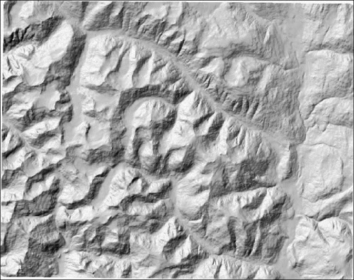
As you can see, the preceding image is much easier to comprehend than the original pseudo-color representation we examined originally. Next, let's look at the slope raster used to create the shaded relief:
The slope shows the gradual decline in elevation from high points to low points in all directions of the data set. Slope is an especially useful input for many types of hydrology models.
The aspect shows the maximum rate of downslope change from one cell to its neighbors. If you compare the aspect image to the shaded relief image you can see the red and gray values of the aspect image correspond to shadows in the shaded relief. So the slope is primarily responsible for turning the DEM into a terrain relief while the aspect is responsible for the shading.

In the next post, we'll use the elevation data to create elevation contours!

Wednesday, December 4, 2013

Python and Elevation Data: ASCII Grid Files

Editor's Note: This multi-part series is based on Chapter 7 of "Learning Geospatial Analysis with Python" and republished with permission from Packt Publishing. This series will cover using Python to work with elevation data.  


Introduction

Elevation data is one of the most fascinating types of geospatial data. It represents many different types of
Image courtesy of the
US National Park Service
data sources and formats. Elevation data can display properties of both vector and raster data resulting in unique data products. Elevation data can serve the following purposes:
  • Terrain visualization
  • Land cover classification
  • Hydrology modelling
  • Transportation routing
  • Feature Extraction
You can't perform all of these options with both raster and vector data but because elevation data is three dimensional, containing x, y, and z coordinates, you can often get more out of these data than any other type.

In this chapter, we're going to learn to read and write elevation data in both raster and vector point formats. We'll also create some derivative products. The topics we'll cover are:
  • ASCII Grid elevation data files
  • Shaded-relief images
  • Elevation contours
  • Gridding LIDAR data
  • Creating a 3D mesh
Editor's Note:  This post will cover ASCII Grid elevation data files.  Each bullet above will be a separate post in this series. Instructions for installing GDAL and its Python bindings can be found here: http://goo.gl/WVPd1n.  On most linux systems you can run: apt-get install python-gdal. In my book I provide detailed instructions and links for Windows/Mac/Linux.  On all platforms PIL and Numpy can be installed using Python SetupTools through easy_install or pip.

For most of this chapter we'll use ASCII Grid files or ASCIIGRID . These files are a type of raster data usually associated with elevation data. This grid format stores data as text in equally sized square rows and columns with a simple header. Each cell in a row/column stores a single numeric value, which can represent some feature of terrain, such as elevation, slope, or flow direction. The simplicity makes it an easy-to-use, platform independent raster format. This format is described in the ASCII GRIDS section in Chapter 2, Geospatial Data.

Throughout the book we've relied on GDAL and to some extent PIL to read and write geospatial raster data including the gdalnumeric module to load raster data into NumPy arrays. But ASCIIGRID allows us to read and write rasters using only Python or even NumPy.
Tip: As a reminder, some elevation data sets use image formats to store elevation data. Most image formats only support 8-bit values ranging between 0-255; however, some formats, including TIFF, can store larger values. Geospatial software can typically display these data sets; however, traditional image software and libraries usually do not. For simplicity in this chapter, we'll stick to the ASCIIGRID format for data, which is both human and machine readable, as well as being widely supported.

Reading grids

NumPy has the ability to read the ASCIIGRID format directly using its loadtxt() method designed to read arrays from text files. The first six lines consist of the header, which are not part of the array. The following lines are a sample of a grid header:

ncols        250
nrows        250
xllcorner    277750.0
yllcorner    6122250.0
cellsize     1.0
NODATA_value      -9999

Line 1 contains the number of columns in the grid, which is synonymous with the x axis. Line 2 represents the y axis described as a number of rows. Line 3 represents the x coordinate of the lower left corner, which is the minimum x value. Line 4 is the corresponding minimum y value in the lower left corner of the grid. Line 5 is the cell size or resolution of the raster. Because the cells are square, only one size value is needed, as opposed to the separate x and y resolution values in most geospatial rasters. The fifth line is no data value, which is a number assigned to any cell for which a value is not provided. Geospatial software ignores these cells for calculations and often allows special display settings for it, such as coloring them black. The value -9999 is a common no data placeholder value used in the industry, which is easy to detect in software. In some examples, we'll use the number zero; however, zero can often also be a valid data value.

The numpy.loadtxt() method includes an argument called skiprows , which allows you to specify a number of lines in the file to be skipped before reading array values. To try this technique out you can download a sample grid file called myGrid.asc at the following URL:

https://geospatialpython.googlecode.com/files/myGrid.asc

So for myGrid.asc we would use the following code:

myArray  = numpy.loadtxt("myGrid.asc", skiprows=6)

This line results in the variable myArray containing a numpy array derived from the ASCIIGRID file myGrid.asc. The ASC file name extension is used by the ASCIIGRID format. This code works great but there's one problem. NumPy allows us to skip the header but not keep it. And we need to keep it to have a spatial reference for our data for processing, as well as for saving this grid or creating a new one.

To solve this problem we'll use Python's built-in linecache module to grab the header. We could open the file, loop through the lines, store each one in a variable, and then close the file. But linecache reduces the solution to a single line. The following line reads the first line in the file into a variable called line 1:

import linecache
line1 = linecache.getline("myGrid.asc", 1)

In the examples in this chapter we'll use this technique to create a simple header processor that can parse these headers into python variables in just a few lines.

Writing grids

Writing grids in Numpy is just as easy as reading them. We use the corresponding numpy.savetxt() function to save a grid to a text file. The only catch is, we must build and add the six lines of header information before we dump the array to the file. This process is slightly different depending on if you are using NumPy versions before 1.7 or after. In either case, you build the header as a string first. If you are using NumPy 1.7 or later, the savetext() method has an optional argument called header, which lets you specify a string as an argument. You can quickly check your NumPy version from the command line using the following command:

python -c "import numpy;print numpy.__version__" 
1.6.1

The backwards compatible method is to open a file, write the header then dump the array. Here is a sample of the Version 1.7 approach to save an array called myArray to an ASCIIGRID file called myGrid.asc:


header = "ncols     %s\n" % myArray.shape[1]
header += "nrows    %s\n" % myArray.shape[0]
header += "xllcorner 277750.0\n"
header += "yllcorner 6122250.0\n"
header += "cellsize 1.0\n"
header += "NODATA_value -9999\n"

numpy.savetxt("myGrid.asc", myArray, \
header=header, fmt="%1.2f")

We make use of python format strings, which allow you to put placeholders in a string to format python objects to be inserted. The %s format variable turns whatever object you reference into a string. In this case we are referencing the number of columns and rows in the array. In NumPy, an array has both a size and shape property. The size property returns an integer for the number of values in the array. The shape property returns a tuple with the number of rows and columns, respectively. So, in the preceding example, we use the shape property tuple to add the row and column counts to the header of our ASCII Grid. Notice we also add a trailing newline character for each line (\n). There is no reason to change the x and y values, cell size, or nodata value unless we altered them in the script. The savetxt() method also has a fmt argument, which allows you to use Python format strings to specify how the array values are written. In this case the %1.2f value specifies floats with at least one number and no more than two decimal places.

The backwards compatible version for NumPy, before 1.6, builds the header string in the same way but creates the file handle first:

import numpy
f = open("myGrid.asc", "w")
f.write(header)
numpy.savetxt(f, myArray, fmt="%1.2f")
f.close()

In the examples in this chapter, we'll introduce Python with an approach for writing files, which provides more graceful file management by ensuring files are closed properly. If any exceptions are thrown, the file is still closed cleanly:

with open("myGrid.asc", "w") as f:
    f.write(header)
    numpy.savetxt(f, myArray, fmt="%1.2f")

As you'll see in the upcoming examples, this ability to produce valid geospatial data files using only NumPy is quite powerful. In the next couple of examples we'll be using an ASCIIGRID Digital Elevation Model (DEM) of a mountainous area near Vancouver, British Columbia in Canada. You can download this sample as a ZIP file at the following URL:

https://geospatialpython.googlecode.com/files/dem.zip

The following image is the raw DEM colorized using QGIS with a color ramp that makes lower elevation values dark blue and higher elevation values bright red:

While we can conceptually understand the data this way, it is not an intuitive way to visualize the data. Let's see if we can do better.  In the next post we'll create a shaded relief image using this data.

Tuesday, November 26, 2013

Extracting Features from Images

Editor's Note: Republished from "Learning Geospatial Analysis with Python" with permission from Packt Publishing. This post is a follow-on to the previous post "Image Classification with Numpy and GDAL"

The ability to classify an image leads us to another remote-sensing capability. Vector GIS data such as shapefiles are typically extracted from remotely-sensed images. Extraction normally involves an analyst clicking around each object in an image and drawing the feature to save it as data. But it is also possible with good remotely-sensed data and proper pre-processing to automatically extract features from an image.

For this example we'll take a subset of our Landsat 8 thermal image to isolate a group of barrier islands as seen in the following screenshot:

You can download this image here:

http://geospatialpython.googlecode.com/files/islands.zip

Our goal with this example is to automatically extract the three islands in the image as a shapefile. But before we can do that, we need to mask out any data we aren't interested in. For example, the water has a wide range of pixel values, as do the islands themselves. If we just want to extract the islands themselves, we need to push all pixel values into just two bins to make the image black and white. This technique is called thresholding . The islands in the image have enough contrast with the water in the background such that thresholding should isolate them nicely.

In the following script we will read the image into an array and then histogram the image using only two bins. We will then use the colors black and white to color the two bins. This script is simply a modified version of our classification script with a very limited output:

import gdalnumeric

# Input file name (thermal image)
src = "islands.tif"

# Output file name
tgt = "islands_classified.tiff"

# Load the image into numpy using gdal
srcArr = gdalnumeric.LoadFile(src)

# Split the histogram into 20 bins as our classes
classes = gdalnumeric.numpy.histogram(srcArr, bins=2)[1]

lut = [[255,0,0],[0,0,0],[255,255,255]]

# Starting value for classification
start = 1

# Set up the output image
rgb = gdalnumeric.numpy.zeros((3, srcArr.shape[0], \
   srcArr.shape[1],),gdalnumeric.numpy.float32)
       
# Process all classes and assign colors
for i in range(len(classes)):
    mask = gdalnumeric.numpy.logical_and(start <= srcArr, \ 
    srcArr <= classes[i])
    for j in range(len(lut[i])):
        rgb[j] = gdalnumeric.numpy.choose(mask, (rgb[j], \
        lut[i][j]))
    start = classes[i]+1 

# Save the image
gdalnumeric.SaveArray(rgb.astype(gdalnumeric.numpy.uint8), \
 tgt, format="GTIFF", prototype=src)
 
The output looks great as seen in the following screenshot:


The islands are clearly isolated so our extraction script will be able to identify them as polygons and save them to a shapefile. The GDAL library has a method called Polygonize() that does exactly that. It groups all sets of isolated pixels in an image and saves them out as a feature data set. One interesting technique we will use in this script is to use our input image as a mask. The Polygonize() method allows you to specify a mask that will use the color black as a filter that will prevent the water from being extracted as a polygon, so we'll end up with just the islands. Another area to note in the script is that we copy the georeferencing information from our source image to our shapefile to geolocate it properly:

import gdal
import ogr, osr

# Thresholded input raster name
src = "islands_classified.tiff"
# Output shapefile name
tgt = "extract.shp"
# OGR layer name
tgtLayer = "extract"
# Open the input raster
srcDS = gdal.Open(src)
# Grab the first band
band = srcDS.GetRasterBand(1)
# Force gdal to use the band as a mask
mask = band
# Set up the output shapefile
driver = ogr.GetDriverByName("ESRI Shapefile")
shp = driver.CreateDataSource(tgt)
# Copy the spatial reference
srs = osr.SpatialReference()
srs.ImportFromWkt(srcDS.GetProjectionRef())
layer = shp.CreateLayer(tgtLayer, srs=srs)
# Set up the dbf file
fd = ogr.FieldDefn( "DN", ogr.OFTInteger )
layer.CreateField(fd)
dst_field = 0
# Automatically extract features from an image!
extract = gdal.Polygonize(band, mask, layer, dst_field, [], None)
 
The output shapefile is simply called extract.shp. We'll bring that script back here to look at our shapefile, but we'll add something to it. The largest island has a small lagoon which shows up as a hole in the polygon. In order to properly render it, we have to deal with parts in a shapefile record. The previous example using that script did not do that, so we'll add that piece as we loop through the shapefile features. The code comments in the following code outline the technique.  You can download the pure Python PNGCanvas module from the Tao of Mac website:

import shapefile
import pngcanvas
# Open the extracted islands
r = shapefile.Reader("extract.shp")
# Setup the world to pixels conversion
xdist = r.bbox[2] - r.bbox[0]
ydist = r.bbox[3] - r.bbox[1]
iwidth = 800
iheight = 600
xratio = iwidth/xdist
yratio = iheight/ydist
polygons = []
# Loop through all shapes
for shape in r.shapes():
  # Loop through all parts to catch
  # polygon holes!
  for i in range(len(shape.parts)):
    pixels=[]
    pt = None
    if I < len(shape.parts)-1:
      pt = shape.points[shape.parts[i]:shape.parts[i+1]]
    else:
      pt = shape.points[shape.parts[i]:]
    for x,y in pt:
      px = int(iwidth - ((r.bbox[2] - x) * xratio))
      py = int((r.bbox[3] - y) * yratio)
      pixels.append([px,py])
    polygons.append(pixels)
# Set up the output canvas
c = pngcanvas.PNGCanvas(iwidth,iheight)
# Loop through the polygons and draw them
for p in polygons:
  c.polyline(p)
# Save the image
f = file("extract.png", "wb")
f.write(c.dump())
f.close()
 
The following screenshot shows our automatically extracted island features! Commercial packages that do this kind of work can easily cost tens of thousands of dollars. While these packages are very robust, it is still fun to see how far you can get with simple Python scripts and a few open source packages. In many cases you can do everything you need to do.
 
 
 The western-most island contains the polygon hole as shown in the following screenshot, which is zoomed to that area:
 
 
Automated feature extraction is a holy grail within geospatial analysis because of the cost and tedious effort required to manually extract features. The key to feature extraction is proper image classification. Automated feature extraction works well with water bodies (and islands), roads, farm fields, buildings, and other features that tend to have high-contrast pixel values with their background.

Friday, November 22, 2013

Image Classification with Numpy and GDAL

Editor's Note:  This post is published with permission from Packt Publishing and originally published in my book. 

Automated Remote Sensing ( ARS ) is rarely ever done in the visible spectrum. The most commonly available wavelengths outside of the visible spectrum are infrared and near-infrared. The following scene is a thermal image (band 10) from a fairly recent Landsat 8 flyover of the US Gulf Coast from New Orleans, Louisiana to Mobile, Alabama. Major natural features in the image are labeled so you can orient yourself:


Because every pixel in that image has a reflectance value, it is information. Python can "see" those values and pick out features the same way we intuitively do by grouping related pixel values. We can colorize pixels based on their relation to each other to simplify the image and view related features. This technique is called classification. Classifying can range from fairly simple groupings based only on some value distribution algorithm derived from the histogram to complex methods involving training data sets and even computer learning and artificial intelligence. The simplest forms are called unsupervised classifications, whereas methods involving some sort of training data to guide the computer are called supervised. It should be noted that classification techniques are used across many fields, from medical doctors trying to spot cancerous cells in a patient's body scan, to casinos using facial-recognition software on security videos to automatically spot known con-artists at blackjack tables.
 
To introduce remote sensing classification we'll just use the histogram to group pixels with similar colors and intensities and see what we get. First you'll need to download the Landsat 8 scene here:
 
 
Instead of our histogram() function from previous examples, we'll use the version included with NumPy that allows you to easily specify a number of bins and returns two arrays with the frequency as well as the ranges of the bin values. We'll use the second array with the ranges as our class definitions for the image. The lut or look-up table is an arbitrary color palette used to assign colors to classes. You can use any colors you want.
 
Note: In the following code we use the gdalnumeric module which allows Numpy and GDAL to work together.  GDAL reads compatible image/data formats and converts them to Numpy arrays.  The Numpy module was formerly called Numeric. 
 
import gdalnumeric

# Input file name (thermal image)
src = "thermal.tif"

# Output file name
tgt = "classified.jpg"

# Load the image into numpy using gdal
srcArr = gdalnumeric.LoadFile(src)

# Split the histogram into 20 bins as our classes
classes = gdalnumeric.numpy.histogram(srcArr, bins=20)[1]

# Color look-up table (LUT) - must be len(classes)+1.
# Specified as R,G,B tuples 
lut = [[255,0,0],[191,48,48],[166,0,0],[255,64,64],
[255,115,115],[255,116,0],[191,113,48],[255,178,115],
[0,153,153],[29,115,115],[0,99,99],[166,75,0],
[0,204,0],[51,204,204],[255,150,64],[92,204,204],[38,153,38],
\ [0,133,0],[57,230,57],[103,230,103],[184,138,0]]

# Starting value for classification
start = 1

# Set up the RGB color JPEG output image
rgb = gdalnumeric.numpy.zeros((3, srcArr.shape[0],
srcArr.shape[1],), gdalnumeric.numpy.float32)
       
# Process all classes and assign colors
for i in range(len(classes)):
    mask = gdalnumeric.numpy.logical_and(start <= \
 srcArr, srcArr <= classes[i])
    for j in range(len(lut[i])):
      rgb[j] = gdalnumeric.numpy.choose(mask, (rgb[j], \ 
    lut[i][j]))
    start = classes[i]+1 

# Save the image    
gdalnumeric.SaveArray(rgb.astype(gdalnumeric.numpy.uint8), \
tgt, format="JPEG")

The following image is our classification output, which we just saved as a JPEG. We didn't specify the prototype argument when saving as an image, so it has no georeferencing information:

 
This result isn't bad for a very simple unsupervised classification. The islands and coastal flats show up as different shades of green. The clouds were isolated as shades of orange and dark blues. We did have some confusion inland where the land features were colored the same as the Gulf of Mexico. We could further refine this process by defining the class ranges manually instead of just using the histogram.
 

Thursday, November 7, 2013

Must See: Going Spatial with Python and Github

Check out this lightning talk by the talented Sara Safavi at the Austin, TX PyLadies Meetup:
Spatial Pythonista
Sara Safavi
 http://goo.gl/c3pD5l

And see the rest of her work at: 


Tuesday, November 5, 2013

Geospatial Python - the Book

I'm pleased to announce Packt Publishing officially released my new book "Learning Geospatial Analysis with Python".  Packt already has two other books related to geospatial Python.  All three books are featured on the right-side border of this page.  I went through a great deal of effort to compliment these two existing books with different but relevant information.

My goal for this book is to provide geospatial Python examples with the following priorities:
  1. Use Pure Python examples as much as possible (standard library only, or third party libraries that only use the standard library)
  2. Use PYPI-compatible libraries which can be installed using easy_install or pip
  3. If I must use Python bindings to a third-party compiled library, focus on methods which lack good examples elsewhere and avoid repeating other books and blogs
If you've ever tried to implement even a simple spatial algorithm, you'll find the vast majority of programmers rely on a relatively small set of core libraries.  These libraries are then built up into larger toolkits which tie those libraries together and add additional value.

The following diagram is a high-level summary of the geospatial software ecosystem, and thereby the Python geospatial ecosystem.  The "800-pound gorillas" including GEOS, PROJ.4 and GDAL are the foundation of nearly all other software.  In this diagram the CGAL and JTS libraries are different.  Both CGAL and JTS are the reference implementations for many of the spatial algorithms later used by GEOS:

The geospatial software industry consists of a small handful of open-source
libraries which support the vast majority of all other software, both proprietary
and open-source.

These libraries are:
  1. Actively maintained and free (open source!)
  2. Implement operations and data access complex enough that nobody wants to reinvent the wheel
I have used these libraries for years.  But I am also stubbornly curious.  I like to understand the algorithms inside the proverbial black box.  My favorite way to understand algorithms is through Python.  I do not have a computer science degree or a degree in mathematics.  I am ignorantly dangerous in almost any programming language.

But what I like about Python is the syntax. It is so clean and expressive it makes hard things easier.  I am not alone.  Scores of non-programmer biologists, meteorologists, economists, medical researchers, artists and other specialists have found Python a user-friendly way to model and solve both trivial and complicated real-world problems.  

But there is a large gap in the literature. For any given problem you can almost always find pure algorithms in research papers or implementations in C/C++ libraries.  But rarely can you find working, practical implementations in Python.  Of course many of the compiled libraries are open source but their structure is complex enough that the casual learner must invest a significant amount of time in understanding most of the code base to uncover a given algorithm.  

The most common reason cited for using compiled libraries versus pure Python is that interpreted languages like Python are far too slow to be efficient and useful for most geospatial operations.  I find this reason unsatisfying for the following reasons:
  1. It discredits Python as a learning tool.  There's no need for speed in learning.
  2. As server platforms become increasingly virtualized, multiplied, and abstracted, our view of resource constraints can continually be relaxed in exchange for faster development with more participants 
  3. There are many tools out there which make pure Python faster when you are ready to optimize
  4. As geospatial applications become more task specific, implementing a handful of algorithms instead of using a "kitchen-sink" toolkit becomes desirable
  5. As mobile devices become increasingly important, dragging around a large compiled tool chain becomes less desirable.
  6. When you bind Python to a compiled library, both of which are updated regularly you have an additional maintenance routine supporting multiple platforms.  This issue varies in difficulty but it's never easy.  This group excludes compiled libraries designed specifically for Python (Numpy, PIL, Fiona, Shapely).
  7. To me, Python's greatest value is as a meta-syntax.  The Python C interpreter alone runs on 30+ platforms.  But the Python C interpreter is often called a "reference implementation".  The Python interpreter has been implemented in dozens of other programming languages including Java (Jython) and .NET (IronPython), and Python itself (PyPy).  So why do people go through the trouble to port Python so many places?  Because the programmatic expression allowed by the syntax is just great.  I always liked the metaphor, "Python is executable pseudocode".  The excellent design of the language from a user standpoint is why nearly every geospatial platform, proprietary or open-source, has a Python API as opposed to other options.
I originally wrote the PyShp library to learn more about both Python and Shapefiles.  I kept it simple by releasing a single file using only the standard library.  Since its release PyShp has become extremely popular. It proved to me there is indeed a demand for spatial software written in pure Python without external dependencies.

"Learning Geospatial Analysis with Python" is my humble attempt at laying a plank in the bridge between abstract algorithms and as close to pure Python implementations as I could.  I took the word "learning" seriously.  I don't try to teach Python as a language because that's been done and done well already.  I do explore common geospatial concepts early on and move into algorithms later in the book which are more advanced (and useful!).

So if you're new to geospatial analysis the first few chapters try to ease you into the field from a software and data perspective before switching to Python.  If you're an experienced geospatial developer I included some interesting examples of virtually undocumented features of GDAL in Python as well as examples of using Numpy for operations that are normally handed off to GDAL or or SciPy.  This book contains more examples of Remote Sensing using Python than any book I've come across yet.

The book is available from Amazon, O'Reilly, and Barnes & Noble as both a paperback and all the major eBook formats.  I hope you find it useful and I hope it increases the use of Python for geospatial analysis and applications.


Sunday, October 20, 2013

Editing a Shapefile

The PyShp module allows you to read existing shapefiles and write new shapefiles using its Reader and Writer classes respectively.  Sometimes you add, delete, or change a feature.
Editing a shapefile involves adding, deleting or 
changing features or attributes


The shapefile format is actually designed to allow editing a shapefile by modifying the contents of the shp and dbf file directly and then recreating the shx index file (and any dbf indexes).  This method can be beneficial for extremely large files but it can leave "dead space" in the files when you move bytes around.  Some shapefile libraries may not handle that data correctly.

The cleanest and simplest way to edit a shapefile is to create a shapefile Reader, edit the features as Python objects, move the features and attributes to a Writer object, and then save a new shapefile or just write over the original.

We can demonstrate this technique with a simple polygon shapefile.  The following map image is "Tropical Storm Rick" based on a polygon shapefile downloaded from the US National Weather Service:

You can download the shapefile as a zip file here:

The following example will use the technique outlined above to add a new tropical storm polygon east of Rick named "Stanley":

import shapefile
# Polygon shapefile we are updating.
# We must include a file extension in
# this case because the file name
# has multiple dots and pyshp would get
# confused otherwise.
file_name = "ep202009.026_5day_pgn.shp"
# Create a shapefile reader
r = shapefile.Reader(file_name)
# Create a shapefile writer
# using the same shape type
# as our reader
w = shapefile.Writer(r.shapeType)
# Copy over the existing dbf fields
w.fields = list(r.fields)
# Copy over the existing dbf records
w.records.extend(r.records())
# Copy over the existing polygons
w._shapes.extend(r.shapes())
# Add a new polygon
w.poly(parts=[[[-104,24],[-104,25],[-103,25],[-103,24],[-104,24]]])
# Add a new dbf record for our polygon making sure we include
# all of the fields in the original file (r.fields)
w.record("STANLEY","TD","091022/1500","27","21","48","ep")
# Overwrite the old shapefile or change the name and make a copy 
w.save(file_name)
This script will add a simple square polygon to the shapefile with some attributes matching those of the original shapefile.  The following map image shows the changes:
shapefile example
You can download the script source here:

This same technique is also used in my posts on merging shapefiles and subsetting a shapefile by attributes.

Tuesday, July 23, 2013

Shapefile to GeoJSON

Here's a quick example by Martin Laloux using the new PyShp geo-interface and the built-in json module to convert a shapefile to geojson in pure Python:
 import shapefile
   # read the shapefile
   reader = shapefile.Reader("my.shp")
   fields = reader.fields[1:]
   field_names = [field[0] for field in fields]
   buffer = []
   for sr in reader.shapeRecords():
       atr = dict(zip(field_names, sr.record))
       geom = sr.shape.__geo_interface__
       buffer.append(dict(type="Feature", \
        geometry=geom, properties=atr)) 
   
   # write the GeoJSON file
   from json import dumps
   geojson = open("pyshp-demo.json", "w")
   geojson.write(dumps({"type": "FeatureCollection",\
    "features": buffer}, indent=2) + "\n")
   geojson.close()

Wednesday, June 26, 2013

Dots in Shapefile Names

I came across a post from another blogger recently which highlighted an issue I hadn't considered before.  Most operating systems allow for an arbitrary number of periods "." in a file name.  For example your shp file in a shapefile set might be named "cities.2013.v.1.2.shp".  While I'm aware of that fact I did not really take it into consideration when designing PyShp.  Here are some factors I did consider:
1. There are at least 3 and up to 9 file types in a single shapefile data set.
2. Dbf files are a fairly common data format for file-based databases.
3. The shx file is just an index and does not contain critical data.

Given these considerations I made it possible to just specify the the base name of a shapefile when reading or writing or you can add an extension IF you want.  Pyshp doesn't rely on the extension.  So in the above example I could just use "cities.2013.v.1.2" in theory.  

That way if one of the files was missing or for some reason you had no control over how the file name was passed to your program the software would just work.  I figured this approach would be the most robust and intuitive, user-friendly method.  In fact if you DO specify a file extension PyShp just chops is off to get the base name using Python's os.path.splitext() module method and then rebuilds the requisite file names before checking to see if they even exist.

There's only one problem.  If you use the base file name AND you have extra dots in your file name as in the example, Python still chops off everything after the last dot assuming it is the file extension.  This functionality is fair since there's no way programatically to be sure what is an extension and what is not.  You could use a look-up table in this context but that can lead to other problems.  So in the above example if you pass the base file name to the PyShp Reader object the base name would be shortened to "cities.2013.v.1" which would result in IO exceptions.

The safe workaround is to just always include a three-letter extension in the file name if you might have dots. I may eventually try to program around this but it's kind of a corner case with a reasonable workaround.  

Sunday, June 23, 2013

PyShp Version 1.1.7 Release

PyShp 1.1.7 is out after several months of virtually no updates.  This release fixes a bunch of minor issues
plus a couple of important features.  You can get it through setuptools or source from the CheeseShop: https://pypi.python.org/pypi/pyshp/1.1.7.  The Google Code page is here:https://code.google.com/p/pyshp/

And as usual there are no dependencies other than Python itself.  Updates include:
  • Added Python geo_interface convention to export shapefiles as GeoJSON.
  • Used is_string() method to detect file names passed as unicode strings (failed on unicode strings before).
  • Added Reader.iterShapes() method to iterate through geometry records for parsing large files efficiently.
  • Added Reader.iterRecords() method to iterate through dbf records efficiently in large files.
  • Modified shape() method to use iterShapes() if shx file is not available as well as record() method.
  • Fixed bug which prevents writing the number 0 to dbf fields.
  • Updated shape() method to calculate and seek the start of the next record. The shapefile spec does not require the content of a geometry record to be as long as the content length defined in the header. The result is you can delete features without modifying the record header allowing for empty space in records.
  • Added enforcement of closed polygons in the Writer.poly() method.

  • Added unique file name generator to use if no file names are passed to a writer instance when saving (ex. w.save()). The unique file name is returned as a string.
  • Updated "bbox" property documentation to match Esri specification.
The __geo_interface__ update required a polygon area calculator.  This method is undocumented but you can feed a list of points representing a polygon to shapefile.signed_area(coords) and get an area calculation back. If the area is a positive number the points are clockwise (outer ring).  If the area is negative then the points are in counter-clockwise order (i.e. an inner polygon ring).

Monday, May 20, 2013

New __geo_interface__ for PyShp


Christian Ledermann took the initiative to fork pyshp and add the __geo_interface__ convention.
http://twitter.com/GeoJSON


The __geo_interface__ is a community standard riding the current "less is more" entropy wave to get away from heavy data exchange standards, make software compatible, and get some work done.

This standard is very pythonic and well thought out which is no surprise because Sean Gillies and Howard Butler are a driving forces behind it.  The goal is to make moving data around among libraries with different specialties, like Shapely and PySAL, easier.  It is closely tied to GeoJSON which is getting a lot of traction and shaking up the industry and community.

Christian's  __geo_interface__ implementation for PyShp is here:

https://github.com/cleder/pyshp

He also wrote some ogr2ogr-style conversion samples to show you how to use it here:
https://github.com/cleder/geo_file_conv

I'm 100% behind these ideas and will roll this interface into the main trunk.  But there's nothing stopping you from using Christian's fork today.

Enjoy!

Tuesday, April 9, 2013

Add a Field to an Existing Shapefile

The dbf file of a shapefile is a simple file-based database with rows and columns.  The rows are
Adding a field where there wasn't one before has
limitless possibilities.
"records" and the columns are "fields".  Sometimes you want to add an additional field to the dbf file to capture some new type of information not originally included.

Today's example shows you how to use pyshp to add a new field to an existing shapefile.  This operation is a two-step process.  You must first update the dbf header to define the new field.  Then you must update each record to account for a new column in the database so everything is balanced.

In the past, I've demonstrated modifying existing shapefiles for other reasons including merging shapefiles and deleting features in shapefiles.  In every case you are actually reading in the existing shapefile, creating a new shapefile in memory and then writing out the new file either separately or on top of the old one.  Even in really high-end GIS packages that's basically all you're doing.  Some packages will use a temporary file in between. 

Here's the example.  We'll create a counter that gives us unique sample data to append to each record just so we can see the changes clearly.  In the real world, you'd probably just insert a blank palce holder.

import shapefile

# Read in our existing shapefile
r = shapefile.Reader("Mississippi")

# Create a new shapefile in memory
w = shapefile.Writer()

# Copy over the existing fields
w.fields = list(r.fields)

# Add our new field using the pyshp API
w.field("KINSELLA", "C", "40")

# We'll create a counter in this example
# to give us sample data to add to the records
# so we know the field is working correctly.
i=1

# Loop through each record, add a column.  We'll
# insert our sample data but you could also just
# insert a blank string or NULL DATA number
# as a place holder
for rec in r.records():
 rec.append(i)
 i+=1
 # Add the modified record to the new shapefile 
 w.records.append(rec)

# Copy over the geometry without any changes
w._shapes.extend(r.shapes())

# Save as a new shapefile (or write over the old one)
w.save("Miss") 

So there you have it. Overall it's a pretty simple process that can be extended to do some sophisticated operations.  The sample Mississippi shapefile can be found here.  But this shapefile only has one record so it's not that interesting.  But it's lightweight and easy to examine the dbf file in your favorite spreadsheet program.