Rasterizing Shapefiles 2: Pure Python

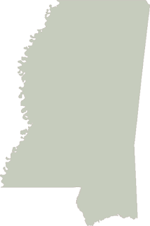
Rasterized shapefile output by PNGCanvas

In my previous post titled "Rasterizing Shapefiles" I used the Python Shapefile Library and the Python Imaging Library to convert a shapefile to an image.  In this post we'll do the same thing again except instead of the C-based PIL we'll use a pure-python library capable of creating PNG images. The library is called "PNGCanvas" and is developed by Rui Carmo at Tao of Mac. Carmo originally created the library as a way to create  sparklines from Python.  From what I've seen the PNGCanvas goes a good bit beyond this simple graphing capability and is commonly used for much more complex jobs.  It works great for rasterizing shapefiles.  PNGCanvas draws irregular polygons perfectly however there is no convenience method to fill anything beyond a rectangle. This functionality could be built on top of PNGCanvas.  The hard part is writing compliant PNGs which is what this library provides.  PNGCanvas has been used on Google App Engine and should work on any hosting system or other platform which provides the native zlib and struct modules.

As I mentioned in the other post this functionality is the basis for web mapping servers but could also be used to quickly generate image renderings of shapefiles for documents, presentations, e-mail, or metadata catalogs.

You'll notice this script is very similar to the PIL script I posted.  Swapping out PIL with PNGCanvas required minimal changes.  As I did last time I also create a world file which allows this image to be layered in most GIS systems albeit only at a single scale.

import shapefile
import pngcanvas

# Read in a shapefile and write png image
r = shapefile.Reader("mississippi")
xdist = r.bbox[2] - r.bbox[0]
ydist = r.bbox[3] - r.bbox[1]
iwidth = 400
iheight = 600
xratio = iwidth/xdist
yratio = iheight/ydist
pixels = []
#
# Only using the first shape record
for x,y in r.shapes()[0].points:
  px = int(iwidth - ((r.bbox[2] - x) * xratio))
  py = int((r.bbox[3] - y) * yratio)
  pixels.append([px,py])
c = pngcanvas.PNGCanvas(iwidth,iheight)
c.polyline(pixels)
f = file("mississippi.png","wb")
f.write(c.dump())
f.close()
#
# Create a world file
wld = file("mississippi.pgw", "w")
wld.write("%s\n" % (xdist/iwidth))
wld.write("0.0\n")
wld.write("0.0\n")
wld.write("-%s\n" % (ydist/iheight))
wld.write("%s\n" % r.bbox[0])
wld.write("%s\n" % r.bbox[3])
wld.close

You can download the shapefile used in this example here:
http://geospatialpython.googlecode.com/files/Mississippi.zip


You can download the script featured above here:
http://geospatialpython.googlecode.com/svn-history/r5/trunk/PureShp2Img.py

Subsetting a Shapefile by Attributes

If you want to select only certain features in one shapefile and export them to another you have two options.  You can select features spatially or by the database attributes.  You can subset by attributes using the Python Shapefile Library in just a few lines of code.  In this example I use a building footprint shapefile which spans three counties and extract building footprints from just one of the counties.  The county name is one of the attributes.  The first step is to create a shapefile reader for the original 41 megabyte building footprint shapefile, Next we create a shapefile writer as a target for extracted features.  We copy the database fields from the first shapefile to the second.  We then make the selection based on attributes.  Next the features in this selection are added to the writer.  Finally the new the shapefile is written.

import shapefile

# Create a reader instance
r = shapefile.Reader("Building_Footprint")
# Create a writer instance
w = shapefile.Writer(shapeType=shapefile.POLYGON)
# Copy the fields to the writer
w.fields = list(r.fields)
# Grab the geometry and records from all features 
# with the correct county name 
selection = [] 
for rec in enumerate(r.records()):
   if rec[1][1].startswith("Hancock"):
      selection.append(rec) 
# Add the geometry and records to the writer
for rec in selection:
   w._shapes.append(r.shape(rec[0]))
   w.records.append(rec[1])
# Save the new shapefile
w.save("HancockFootprints") 

I originally used python list comprehensions for the two loops in this example.  They usually run faster than "for" loops. However some basic testing showed them to be about the same speed in this case and a little harder to read.  If your selection were more complex you probably want to use a for loop anyway to select by multiple attributes or other filters.

As usual the code for this example can be found on the "geospatialpython" Google Code project in the source tree. The shapefile can be found on the same site in the download section.

Rasterizing Shapefiles

Converting a shapefile into an image has two common uses.  The first is in web mapping servers.  All data in the map is fused into an image which is then optionally tiled and cached at different scales.  This method is how Google Maps, ESRI ArcGIS Server, and UMN Mapserver all work.  UMN Mapserver even includes a command-line utility called "Shp2Image" which converts its "mapscript" configuration file into an image for quick testing.  The second common reason to convert a shapefile into an image is to use it as a mask to clip remotely-sensed imagery.  In both cases most geospatial software packages handle these operations for you behind the scenes.

The very simple script below shows you how you can rasterize a shapefile using the Python Shapefile Library (PSL) and the Python Imaging Library (PIL).  PIL is a very old and well-developed library originally created to process remote sensing imagery however it has absolutely no spatial capability.  What it does have is the ability to read and write multiple image formats and can handle very large images.  It also has an API that lets you easily import and export data to and from other libraries using python strings and arrays.  The PIL ImageDraw module provides an easy way to draw on an image canvas.

The following script reads in a shapefile, grabs the points from the first and only polygon, draws them to an image, and then saves the image as a PNG file with an accompanying .pgw world file to make it a geospatial image.   Most modern GIS packages handle PNG images but you could just as easily change the file and worldfile extension to jpg and jgw respectively for even better compatibility. As usual I created minimal variables to keep the code short and as easy to understand as possible.

import shapefile
import Image, ImageDraw

# Read in a shapefile
r = shapefile.Reader("mississippi")
# Geographic x & y distance
xdist = r.bbox[2] - r.bbox[0]
ydist = r.bbox[3] - r.bbox[1]
# Image width & height
iwidth = 400
iheight = 600
xratio = iwidth/xdist
yratio = iheight/ydist
pixels = []
for x,y in r.shapes()[0].points:
  px = int(iwidth - ((r.bbox[2] - x) * xratio))
  py = int((r.bbox[3] - y) * yratio)
  pixels.append((px,py))
img = Image.new("RGB", (iwidth, iheight), "white")
draw = ImageDraw.Draw(img)
draw.polygon(pixels, outline="rgb(203, 196, 190)", 
                fill="rgb(198, 204, 189)")
img.save("mississippi.png")

# Create a world file
wld = file("mississippi.pgw", "w")
wld.write("%s\n" % (xdist/iwidth))
wld.write("0.0\n")
wld.write("0.0\n")
wld.write("-%s\n" % (ydist/iheight))
wld.write("%s\n" % r.bbox[0])
wld.write("%s\n" % r.bbox[3])
wld.close  

You can download this script here:
http://geospatialpython.googlecode.com/svn/trunk/shp2img.py

You can download the shapefile used here:
http://geospatialpython.googlecode.com/files/Mississippi.zip

Of course you will also need the Python Shapefile Library found here and the latest version of the Python Imaging Library from here.

The image created by this script is featured at the top of this post.

The idea of using a shapefile as a clipping mask for an image can be done with GDAL.   The python API for GDAL includes integration with the well-known Python Numeric (NumPy) package using a module called "gdalnumeric".  Both gdalnumeric and PIL contain "tostring" and "fromstring" methods which allow you to move image data back and forth between the packages.  GDAL and NumPy make handling geospatial data as numerical arrays easier and PIL's API makes creating a polygon clipping mask much easier.

I'll cover using PIL, GDAL, NumPy, and PSL together in a future post. I'll also demonstrate a way where the above operation can be performed using pure Python.

Dot Density Maps with Python and OGR

If you use Python for GIS sooner or later you'll use GDAL for manipulating raster data and its vector cousin OGR for working with vector data. OGR has a Python API for most of the methods in the C++ library and even provides some basic geometry analysis. And most importantly it can read/write and therefore convert data in a variety of vector file and database formats.

OGR provides a fast way to create dot density maps.  A dot density map represents statistical information about an area as mathematically distributed points. Areas with higher values have a higher concentration of points. This is one of my favorite types of maps because it is a great example of GIS - visualizing geographic data in a way that is instantly comprehensible.

I'm using OGR in this example because it can read and write shapefiles. But unlike the Python Shapefile Library it can also perform basic geometry operations needed for this sample. Most GIS programs would display the population information on some type of memory layer instead of actually outputting a shapefile for the density layer as demonstrated here.  But we're going to keep things simple for this example and just create a shapefile.

Assuming you have Python installed, here are some basic gdal/ogr installation instructions.
1. Go to http://trac.osgeo.org/gdal/wiki/DownloadingGdalBinaries and download the gdal binary for your platform
2. Extract the directory to your hard drive
3. Add the "bin" directory within the gdal folder to your system shell path
4. Set the path to the "data" directory in the gdal folder to an environment variable called "GDAL_DATA"
5. Install the appropriate python module for your Python version and platform from here: http://pypi.python.org/pypi/GDAL/1.6.0#downloads

If you want to follow along with the example below you can download the source shapefile:
http://pyshp.googlecode.com/files/GIS_CensusTract.zip

The end result of this demo is pictured above with both the input census block and output dot density shapefiles. 

The following code will read in the source shapefile, calculate the number of points needed to represent the population density evenly, and then create the point shapefile:

from osgeo import ogr
import random
# Open shapefile, get OGR "layer", grab 1st feature
source = ogr.Open("GIS_CensusTract_poly.shp")
county = source.GetLayer("GIS_CensusTract_poly")
feature = county.GetNextFeature()
# Set up the output shapefile and layer
driver = ogr.GetDriverByName('ESRI Shapefile')
output = driver.CreateDataSource("PopDensity.shp")
dots = output.CreateLayer("PopDensity", geom_type=ogr.wkbPoint)
while feature is not None:
  field_index = feature.GetFieldIndex("POPULAT11")
  population = int(feature.GetField(field_index))
  # 1 dot = 100 people
  density = population / 100
  # Track dots created
  count = 0   
  while count < density:
    geometry = feature.GetGeometryRef()
    minx, maxx, miny, maxy = geometry.GetEnvelope()
    x = random.uniform(minx,maxx)
    y = random.uniform(miny,maxy)
    f = ogr.Feature(feature_def=dots.GetLayerDefn())
    wkt = "POINT(%f %f)" % (x,y)
    point = ogr.CreateGeometryFromWkt(wkt)
    # Don't use the random point unless it's inside the polygon.
    # It should be close as it's in the bounding box
    if feature.GetGeometryRef().Contains(point):
        f.SetGeometryDirectly(point)
        dots.CreateFeature(f)
        count += 1
    # Destroy C object.
    f.Destroy()
  feature = county.GetNextFeature()
source.Destroy()
output.Destroy()    

There is no error handling in this sample so if you run it multiple times you need delete the output dot density shapefile.

Note that this type of rendering only works when you have one polygon representing each data value. For example you couldn't do this operation with a world country boundary shapefile because islands like Hawaii associated with a country would force an inaccurate representation. For that type of map you need to use a choropleth map.

Also note that when you use OGR for shapefile editing you must specify a "layer" after opening a file. This extra step is necessary because OGR handles dozens of formats, some of which are layered vector formats such as DWG using the same API. Also because OGR is a wrapped C library you have to adjust to explicitly destroying objects and extreme camel casing on method calls usually not found in Python.

OGR and the raster equivalent GDAL are two very powerful libraries which dominate the open source geospatial world. They are also included in several well-known commercial packages thanks to the commercial-friendly MIT license.