New Member added to the PyShp Team

Great news - Nicholas Lederer who works with the University of Washington Applied Physics Laboratory recently joined the committers for PyShp.  He has already made some significant contributions (i.e. bug squashing) to the library in his spare time.   He also has bigger design ideas on how to address some issues to make code maintenance easier as contributors grow. We have also been dealing with some niche but important issues elevation values, dbf header fields, and all-too-common incorrect shapefiles produced by other libraries.

I originally wrote this library because I wanted an easy way to read and write shapefiles in pure Python.  That option simply didn't exist from the time I entered the geospatial field in 2000 until 2004 when I started developing this library in my free time.  Hurricane Katrina slowed down the development tremendously for a few years but by 2010 I had finished it.

In those 10 years since I first started looking for a library like PyShp, Python grew tremendously in popularity but nobody developed this kind of library.  The field of geospatial technology also grew and the technology and standards changed radically but shapefiles still seem to stubbornly persist as the most common way to store and exchange geospatial vector data.

Given the library was still potentially relevant I guessed there were at least 4 other people in the world who had a need to write shapefiles in Python as simply as possible.  It turns out there are hundreds, maybe thousands of people who have this need.  And there is no doubt Python itself is firmly entrenched in geospatial technology in general.

I'm looking forward to this library reaching its full potential through a collaborative effort.  Thanks to everybody who has identified issues, provided patches, and joined in this shared interest.

If you're new to this blog and want to help or be helped be sure to check out:

• Twitter:  (@SpatialPython)
• Geospatail Python on Google Groups
• PyShp Project Site
• Geospatial Python Project Site

Working with Elevation Values in Shapefiles

I've had several questions about working with elevation values in shapefiles.  Awhile back I  posted a brief example in the wiki on the google code project site and felt it should be included here so this information is more visible.


Elevation values, known as "Z" values allow you to create 3-dimensional shapefiles. Working with elevation values in the Python Shapefile Library is easy but requires a step which hasn't been well documented until now. Make sure you are working with at least version 1.0 (revision 24 in the repository) as previous versions have a bug that prevents elevation values from being written properly as well as another bug which occurs when creating certain polygons.

The shapefile specification allows for three types of 3-dimensional shapefiles:

PointZ - a 3D point shapefile, PolylineZ - a 3D line shapefile, and PolygonZ - a 3D polygon shapefile.

The most important thing to remember is to explicitly set the shape type of each record to the correct shape type or it will default to a 2-dimensional shape. Eventually the library will automatically detect the elevation type.

Here is a brief example of creating a PolygonZ shapefile:

import shapefile
w = shapefile.Writer(shapeType=shapefile.POLYGONZ)
# OR you can type
# w = shapefile.Writer(shapeType=15)
w.poly([[[-89.0, 33, 12], [-90, 31, 11], [-91, 30, 12]]], shapeType=15)
w.field("NAME")
w.record("PolyZTest")
w.save("MyPolyZ")

When you read 3D shapefiles the elevation values will be stored separately:

>>>import shapefile
>>>r = shapefile.Reader("MyPolyZ")
>>>r.shapes()[0].points
[[-89.0, 33.0], [-90.0, 31.0], [-91.0, 30.0]]
>>>r.shapes()[0].z
[12, 11, 12]

So remember: explicitly set the shapetype for each shape you add to ensure the z values are maintained. And know that the z values are stored in the "z" property of each shape instead of being integrated with the x,y value lists.

Changing a Shapefile's Type

A polygon, line, and point version of the same shapefile.

Sometimes you want to convert a shapefile from one type to another.  For example you may want to convert a line shapefile to a polygon or a polygon to a point or multipoint shapefile.  There are many reasons for this type of operations ranging from error checking, to special queries, to inconvenient distribution formats.  For example a lot of coastline data is distributed as line data but you may want to convert it to a polygon to estimate coastal erosion using area comparisons between two different dates.

Performing this type of conversion is very straightforward using the Python Shapefile Library.  In fact the conversion is basically a one-off version of the shapefile merge example I wrote about recently.  You read in one shapefile and write the features and records out to another of the correct type.  There are a couple of pitfalls you need to be wary of though.  One is the current version (1.0) of the PSL requires you to explicitly set the shape type of each record if you want to convert them.  The second issue is if you are converting to a single point shapefile where each point feature is a record you must compensate for the imbalance in the dbf records by copying the record from the parent feature for each point.  Instead of dealing with this issue you could simply create a multi-point shapefile where each shape record is allowed to be a collection of points.  Which method you choose depends on what you are trying to do with the output.  The examples below cover both methods.

The example in this post takes a state boundary polygon file and converts it to a line shapefile, then a multipoint shapefile, then a regular point shapefile.  Note the difference between the point shapefile and the line and multipoint examples.

"""
Convert one shapefile type to another 
"""

import shapefile


# Create a line and a multi-point 
# and single point version of
# a polygon shapefile

# The shapefile type we are converting to
newType = shapefile.POLYLINE

# This is the shapefile we are trying
# to convert. In this case it's a
# state boundary polygon file for 
# Mississippi with one polygon and
# one dbf record.
r = shapefile.Reader("Mississippi")

## POLYLINE version
w = shapefile.Writer(newType)
w._shapes.extend(r.shapes())
# You must explicity set the shapeType of each record.
# Eventually the library will set them to the same
# as the file shape type automatically.
for s in w.shapes():
  s.shapeType = newType
w.fields = list(r.fields)
w.records.extend(r.records())
w.save("Miss_Line")

## MULTIPOINT version
newType = shapefile.MULTIPOINT

w = shapefile.Writer(newType)
w._shapes.extend(r.shapes())
for s in w.shapes():
  s.shapeType = newType
w.fields = list(r.fields)
w.records.extend(r.records())
w.save("Miss_MPoint")

## POINT version
newType = shapefile.POINT

w = shapefile.Writer(newType)
# For a single point shapefile
# from another type we
# "flatten" each shape
# so each point is a new record.
# This means we must also assign
# each point a record which means
# records are usually duplicated.
for s in r.shapeRecords():
  for p in s.shape.points:
    w.point(*p)
    w.records.append(s.record)  
w.fields = list(r.fields)
w.save("Miss_Point")

You can download the state boundary polygon shapefile used in the example from the GeospatialPython Google Code Project Downloads section.  You can download the sample script above from the subversion repository of that same project.

And of course the Python Shapefile Library is here.

Clip a Raster using a Shapefile

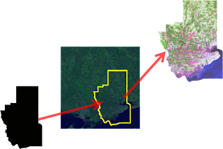
Clipping a satellite image: Rasterize, Mask, Clip, Save

If you read this blog you see most of the material covers shapefiles.  The intent of this blog is to cover remote sensing as well and this article provides a great foundation for remote sensing in Python. In this post I'll demonstrate how to use several Python libraries to to create a script which can take any polygon shapefile and use it as a mask to clip a geospatial image.  Although I'm demonstrating a fairly basic process, this article and the accompanying sample script is densely-packed with lots of good information and tips that would take you hours if not days to piece together reading forum posts, mailing lists, blogs, and trial and error.  This post will get you well on your way to doing whatever you want to do with Python and Remote Sensing.

Satellite and aerial images are usually collected in square tiles more or less the same way your digital camera frames and captures a picture.  Geospatial images are data capturing different wavelengths of light reflected from known points on the Earth or even other planets.  GIS professionals routinely clip these image tiles to a specific area of interest to provide context for vector layers within a GIS map.  This technique may also be used for remote sensing to narrow down image processing to specific areas to reduce the amount of time it takes to analyze the image.

The Process

Clipping a raster is a series of simple button clicks in high-end geospatial software packages.  In terms of computing, geospatial images are actually very large, multi-dimensional arrays.  Remote Sensing at its simplest is performing mathematical operations on these arrays to extract information from the data. Behind the scenes here is what the software is doing (give or take a few steps):

1. Convert the vector shapefile to a matrix which can be used as mask
2. Load the geospatial image into a matrix
3. Throw out any image cells outside of the shapefile extent
4. Set all values outside the shapefile boundary to NODATA (null) values
5. OPTIONAL: Perform a histogram stretch on the image for better visualization
6. Save the resulting image as a new raster.

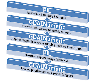
Geospatial Python Raster Clipping Workflow

Tools

Two things I try to do on this blog are build on techniques used in previous posts and focus on pure-Python solutions as much as possible.  The script featured in this post will use one of the shapefile rasterization techniques I've written about in the past.  However I did not go pure-Python on this for several reasons.  Geospatial image formats tend to be extremely complex.  You could make a career out of reading and writing the dozens of evolving image formats out there.  As the old saying goes TIFF stands for "Thousands of Incompatible File Formats".  So for this reason I use the Python bindings for GDAL when dealing with geospatial raster data.  The other issue is the size of most geospatial raster data.  Satellite and high-resolution aerial images can easily be in the 10's to 100's of megabytes size range.  Doing math on these images and the memory required to follow the six step process outlined above exceeds the capability of Python's native libraries in many instances.  For this reason I use the Numpy library which is dedicated to large, multi-dimensional matrix math.  Another reason to use Numpy is tight integration with GDAL in the form of the "GDALNumeric" module. (Numeric was the predecessor to Numpy) In past posts I showed a pure-Python way to rasterize a shapefile.  However I use the Python Imaging Library (PIL) in this example because it provides convenient methods to move data back and forth between Numpy.

Library Installation

So in summary you will need to install the following packages to make the sample script work.  Usually the Python Disutils system (i.e. the "easy_install" script) is the fastest and simplest way to install a Python library.  Because of the complexity and dependencies of some of these tools you may need to track down a pre-compiled binary for your platform.  Both Numpy and GDAL have them linked from their respective websites or the Python Package Index.

• Python Imaging Library
• Numpy
• GDAL

The Example

# RasterClipper.py - clip a geospatial image using a shapefile

import operator
from osgeo import gdal, gdalnumeric, ogr, osr
import Image, ImageDraw

# Raster image to clip
raster = "SatImage.tif"

# Polygon shapefile used to clip
shp = "county"

# Name of clip raster file(s)
output = "clip"

# This function will convert the rasterized clipper shapefile 
# to a mask for use within GDAL.    
def imageToArray(i):
    """
    Converts a Python Imaging Library array to a 
    gdalnumeric image.
    """
    a=gdalnumeric.fromstring(i.tostring(),'b')
    a.shape=i.im.size[1], i.im.size[0]
    return a

def arrayToImage(a):
    """
    Converts a gdalnumeric array to a 
    Python Imaging Library Image.
    """
    i=Image.fromstring('L',(a.shape[1],a.shape[0]),
            (a.astype('b')).tostring())
    return i
     
def world2Pixel(geoMatrix, x, y):
  """
  Uses a gdal geomatrix (gdal.GetGeoTransform()) to calculate
  the pixel location of a geospatial coordinate 
  """
  ulX = geoMatrix[0]
  ulY = geoMatrix[3]
  xDist = geoMatrix[1]
  yDist = geoMatrix[5]
  rtnX = geoMatrix[2]
  rtnY = geoMatrix[4]
  pixel = int((x - ulX) / xDist)
  line = int((ulY - y) / yDist)
  return (pixel, line) 

def histogram(a, bins=range(0,256)):
  """
  Histogram function for multi-dimensional array.
  a = array
  bins = range of numbers to match 
  """
  fa = a.flat
  n = gdalnumeric.searchsorted(gdalnumeric.sort(fa), bins)
  n = gdalnumeric.concatenate([n, [len(fa)]])
  hist = n[1:]-n[:-1] 
  return hist

def stretch(a):
  """
  Performs a histogram stretch on a gdalnumeric array image.
  """
  hist = histogram(a)
  im = arrayToImage(a)   
  lut = []
  for b in range(0, len(hist), 256):
    # step size
    step = reduce(operator.add, hist[b:b+256]) / 255
    # create equalization lookup table
    n = 0
    for i in range(256):
      lut.append(n / step)
      n = n + hist[i+b]
  im = im.point(lut)
  return imageToArray(im)

# Load the source data as a gdalnumeric array
srcArray = gdalnumeric.LoadFile(raster)

# Also load as a gdal image to get geotransform 
# (world file) info
srcImage = gdal.Open(raster)
geoTrans = srcImage.GetGeoTransform()

# Create an OGR layer from a boundary shapefile
shapef = ogr.Open("%s.shp" % shp)
lyr = shapef.GetLayer(shp)
poly = lyr.GetNextFeature()

# Convert the layer extent to image pixel coordinates
minX, maxX, minY, maxY = lyr.GetExtent()
ulX, ulY = world2Pixel(geoTrans, minX, maxY)
lrX, lrY = world2Pixel(geoTrans, maxX, minY)

# Calculate the pixel size of the new image
pxWidth = int(lrX - ulX)
pxHeight = int(lrY - ulY)

clip = srcArray[:, ulY:lrY, ulX:lrX]

# Create a new geomatrix for the image
geoTrans = list(geoTrans)
geoTrans[0] = minX
geoTrans[3] = maxY

# Map points to pixels for drawing the 
# boundary on a blank 8-bit, 
# black and white, mask image.
points = []
pixels = []
geom = poly.GetGeometryRef()
pts = geom.GetGeometryRef(0)
for p in range(pts.GetPointCount()):
  points.append((pts.GetX(p), pts.GetY(p)))
for p in points:
  pixels.append(world2Pixel(geoTrans, p[0], p[1]))
rasterPoly = Image.new("L", (pxWidth, pxHeight), 1)
rasterize = ImageDraw.Draw(rasterPoly)
rasterize.polygon(pixels, 0)
mask = imageToArray(rasterPoly)   

# Clip the image using the mask
clip = gdalnumeric.choose(mask, \
    (clip, 0)).astype(gdalnumeric.uint8)

# This image has 3 bands so we stretch each one to make them
# visually brighter
for i in range(3):
  clip[i,:,:] = stretch(clip[i,:,:])

# Save ndvi as tiff
gdalnumeric.SaveArray(clip, "%s.tif" % output, \
    format="GTiff", prototype=raster)

# Save ndvi as an 8-bit jpeg for an easy, quick preview
clip = clip.astype(gdalnumeric.uint8)
gdalnumeric.SaveArray(clip, "%s.jpg" % output, format="JPEG")

Tips and Further Reading

The utility functions at the beginning of this script are useful whenever you are working with remotely sensed data in Python using GDAL, PIL, and Numpy.

If you're in a hurry be sure to look at the GDAL utility programs.  This collection has a tool for just about any simple operation including clipping a raster to a rectangle.  Technically you could accomplish the above polygon clip using only GDAL utilities but for complex operations like this Python is much easier.

The data referenced in the above script are a shapefile and a 7-4-1 Path 22, Row 39 Landsat image from 2006. You can download the data and the above sample script from the GeospatialPython Google Code project here.

I would normally use the Python Shapefile Library to grab the polygon shape instead of OGR but because I used GDAL, OGR is already there. So why bother with another library?

If you are going to get serious about Remote Sensing and Python you should check out OpenEV.  This package is a complete remote sensing platform including an ERDAS Imagine-style viewer.  It comes with all the GDAL tools, mapserver and tools, and a ready-to-run Python environment.

I've written about it before but Spectral Python is worth a look and worth mentioning again. I also recently found PyResample on Google Code but I haven't tried it yet.  

Beyond the above you will find bits and pieces of Python remote sensing code scattered around the web.  Good places to look are:

• Frank Warmerdam's Blog 
• The GDAL mailing list archives 
• SAGE 
• PyDap 
• PyHDF 
• The SciPy community

More to come!

UPDATE (May 4, 2011): I usually provide a link to example source code and data for instructional posts. I set up the download for this one but forgot to post it.  This zip file contains everything you need to perform the example above except the installation of GDAL, Numpy, and PIL:
http://geospatialpython.googlecode.com/files/clipraster.zip

Make sure the required libraries are installed and working before you attempt this example.  As I mention above the OpenEV package has a Python environment with all required packages except PIL.  It may take a little work to get PIL into this unofficial Python environment but in my experience it's less work than wrangling GDAL into place.

Create a .prj Projection File for a Shapefile

An example of a cordiform map projection a.k.a. 
heart-shaped projection. Happy Valentine's!

If you create a shapefile with ESRI software or receive one from someone who did you may see a ".prj" file included along with the shp, shx, and dbf files.  In fact, the prj file is one of up to 9 possible "official" file extensions for various indexes and other meta files.  Most of these file formats are proprietary.  There are an additional two formats created by the open source community to work around the closed formats created by ESRI for spatial indexing.

The shapefile format does not allow for specifying the map projection of the data. When ESRI created the shapefile format everyone worked with data in only one projection. If you tried to load a layer in a different projection into your GIS weird things would happen.  Not too long ago as hardware capability increased according to Moore's Law, GIS software packages developed the ability to reproject geospatial layers on the fly.  You could now load in layers in any projection and as long as you told the software what projections were involved the map would come together nicely.

ArcGIS 8.x allowed you to manually assign each layer a projection.  This information was stored in the prj file.  The prj file contains a WKT (Well-Known Text) string which has all the parameters for the map projection. So the format is quite simple and was created by the Open GIS Consortium.

But there are several thousand "commonly-used" map projections which were standardized by the European Survey Petroleum Group (EPSG). And there's no way to accurately detect the projection from the coordinates in the shapefile. For these reasons the Python Shapefile Library does not currently handle prj files.

If you need a prj file, the easiest thing to do is write one yourself. The following example creates a simple point shapefile and then the corresponding prj file using the WGS84 "unprojected" WKT.

import shapefile as sf
filename = 'test/point'

# create the shapefile
w = sf.Writer(sf.POINT)
w.point(37.7793, -122.4192)
w.field('FIRST_FLD')
w.record('First','Point')
w.save(filename)

# create the PRJ file
prj = open("%s.prj" % filename, "w")
epsg = 'GEOGCS["WGS 84",'
epsg += 'DATUM["WGS_1984",'
epsg += 'SPHEROID["WGS 84",6378137,298.257223563]]'
epsg += ',PRIMEM["Greenwich",0],'
epsg += 'UNIT["degree",0.0174532925199433]]'
prj.write(epsg)
prj.close()

I've thought about adding the ability to optionally write prj files but the list of "commonly-used" WKT strings is over .5 megs and would be bigger than the shapefile library itself.  I may eventually work something out though.

The easiest thing to do right now is just figure out what WKT string you need for your data and write a file after you save your shapefile. If you need a list of map projection names, epsg codes, and corresponding WKT strings you can download it from the geospatialpython Github "Learn" repository here.

A word of warning if you are new to GIS and shapefiles: the prj file is just metadata about your shapefile.  Changing the projection reference in the prj file will not change the actual projection of the geometry and will just confuse your GIS software.